Everything is Linear Up High, Everything is Curved Down Low: Distributed Representations and the Brain’s Geometry

Blog 2 of a series on Geometry, Topology, and the Future of Machine Learning Representation

---

“The brain does not store the world. It stores the algebra of the world.”

---

Picking Up Where We Left Off

In the first blog of this series, we climbed a ladder of mathematical spaces — from bare topological spaces, through metric and inner product spaces, up to Hilbert spaces of signals — and argued that the dominant paradigm in representation learning is stuck at one rung of that ladder. Current LLMs represent meaning as static points in a finite-dimensional inner product space: real-valued vectors with amplitude but no phase, location but no dynamics.

The natural question that follows is: what should a better representation look like?

The inspiration comes from how the brain does it. The brain’s solution to representation is neither a static vector nor a simple function. It is a distributed algebraic structure — patterns spread across enormous populations of neurons, composed and decomposed by operations that look a lot like the mathematics of signal processing and symbolic algebra.

This blog develops that idea in three acts. First, we ask what geometry high-dimensional data actually has — this is the Manifold Hypothesis, and its implications are stranger than they might seem. Second, we look at how the brain navigates the fundamental tension between generalisation and discrimination, and why it does so with a specific computational circuit that machine learning is only beginning to rediscover. Third, we introduce Vector Symbolic Architectures (VSAs) — a family of frameworks for encoding structured, compositional meaning into distributed representations — and argue that they, more than any other existing formalism, point toward what multimodal generalisation actually requires.

---

Part I: The Geometry of High-Dimensional Data

Cover’s Theorem and the Linearity of High Dimensions

There is a theorem from 1965 that is well-known in the theory of support vector machines but deserves to be much more central to how machine learning practitioners think about representation. Cover’s theorem [1] states:

A pattern classification problem cast into a sufficiently high-dimensional space is more likely to be linearly separable than in a lower-dimensional one.

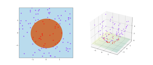
Read that carefully. It is not saying that high-dimensional spaces are easier to work in for some vague reason. It is making a precise geometric claim: if you take a classification problem that is not linearly separable in low dimensions, and you map the data into a sufficiently high-dimensional space (with a nonlinear map), a hyperplane will almost surely suffice. This is the theoretical foundation of kernel methods — the kernel trick implicitly embeds data into a very high-dimensional (often infinite-dimensional) feature space where linear separation becomes possible [2].

The Johnson-Lindenstrauss lemma [3] makes an even stronger statement about what happens in high dimensions: a random projection of \(n\) points from \(\mathbb{R}^d\) into \(\mathbb{R}^k\) (with \(k = O(\log n / \epsilon^2)\)) preserves all pairwise distances up to a factor of \((1 \pm \epsilon)\). This is the core theme behind all the dimensionality reduction techniques. Geometric structure — the shape of the data — survives random projection into high dimensions. You do not need to carefully engineer the high-dimensional space; randomness preserves geometry almost for free.

Together, these results suggest something philosophically interesting: high-dimensional spaces are “more linear.” Complex, curved, tangled relationships in low dimensions tend to become linearly separable when you go up. The nonlinearity is not an intrinsic property of the data — it is a property of the low-dimensional projection you happen to be looking at.

Consider a unit hypercube. The distance from the center to a corner in \(d\) dimensions is \(\frac{\sqrt{d}}{2}\). In 3D, that distance is roughly 0.86.In 1,000D, that distance is approximately 15.8.The corners are “stretching” away into the distance. Simultaneously, the volume of a hypersphere inscribed in that cube shrinks to almost zero relative to the cube. By the time you reach 10 dimensions, the sphere occupies less than 0.25% of the cube’s volume. A reference YouTube video for explanation

The implication is profound: In high dimensions, almost all the volume of a cube is concentrated in its corners. If you were to drop “data points” randomly into this space, they would be so far apart that the concept of a “nearest neighbor” becomes mathematically meaningless. The space is a vast, freezing void of “corners.”

The Manifold Hypothesis: Where the Data Actually Lives

In high-dimensional space, the “Curse of Dimensionality” means that the ambient space is unimaginably vast and mostly empty. If data were distributed uniformly, machine learning would be impossible because we could never collect enough samples to “fill” that space. The Manifold Hypothesis [4] is the observation that nature is “lazy”—it doesn’t use all those corners; it restricts itself to a tiny, structured, curved subset. Images, sounds, and language samples occupy a tiny, curved, low-dimensional manifold embedded within the ambient high-dimensional space. The effective dimensionality of natural images — the number of dimensions you need to account for most of the variance — is far smaller than the pixel count.

This is not just an empirical observation; it follows from the structure of the world. Images of faces are constrained by the geometry of faces: two eyes, a nose, a mouth, all varying continuously with pose, expression, and lighting. The space of valid faces is a manifold parameterised by a handful of continuous variables, embedded in \(\mathbb{R}^{3 \times H \times W}\).

Manifolds have a key geometric property: they are locally Euclidean but globally curved. A small enough neighbourhood of any point on a smooth manifold looks flat — like a patch of \(\mathbb{R}^k\) for some small \(k\). But the global structure can be highly curved, twisted, and topologically complex. A Swiss roll is two-dimensional globally but looks one-dimensional locally if you zoom in far enough along one direction.

This has a direct implication for representation learning:

• In the high-dimensional ambient space: data is sparse, geometry is preserved by random projections, and linear separability is achievable. This is where expansion is useful.
• In the low-dimensional intrinsic space: the manifold has curvature, and a linear map from the ambient space to the intrinsic space will destroy that curvature. You need a nonlinear map — one that “unfolds” the manifold onto a flat coordinate system.

The nonlinearities in deep neural networks are not arbitrary engineering choices. They are the mathematical necessities of mapping a curved low-dimensional manifold onto a flat representational space. A network that is purely linear can only learn linear projections; it cannot unfold a Swiss roll. Rectified linear units, sigmoid functions, and their cousins are the mechanism by which a network “flattens” manifold curvature.

What Current Models Do Well — and What They Miss (Unfolding vs. Expanding)

Modern deep learning systems can be understood as powerful manifold-learning machines. Through successive nonlinear layers, they progressively “unfold” the data manifold. Since small regions are approximately linear, each layer applies local linear transformations that gradually flatten the global structure; it has been confirmed empirically and to some extent theoretically [5, 6].

Large language models extend this idea further. In Transformers, representations evolve layer by layer: a token starts with a lexical embedding and is iteratively refined toward a context-aware meaning. Attention mechanisms guide these updates, determining which parts of the representation space are relevant at each step.

This framework explains much of their success.

However, there is an important limitation.

Manifold learning is fundamentally a compression strategy. It focuses on discovering low-dimensional, invariant structure—capturing what generalizes across variations. This is extremely powerful, but it emphasizes abstraction over distinction.

What it does not naturally provide is the complementary capability: high-dimensional expansion for precise discrimination and compositional structure.

This is where Cover’s Theorem becomes relevant again. It tells us that even if the data manifold remains complex and entangled, projecting it into a sufficiently high-dimensional space makes different points sparse and, therefore, easier to separate linearly. In other words, expansion enables fine-grained discrimination.

So we are left with two complementary needs:

• Unfolding (via nonlinear transformations): to capture structure and enable generalization
  
• Expanding (via high-dimensional representations): to preserve separability and precision

Current models are exceptionally good at the first. They compress, abstract, and generalize. But relying on compression alone risks losing the fine distinctions needed for precise reasoning and compositionality.

To build systems that both generalize and discriminate effectively, we need a balance between these two strategies.

This naturally raises a deeper question: how does the brain achieve this balance?

---

Part II: The Brain’s Circuit — Expansion, Compression, and the Loop Between Them

The Fundamental Circuit

The brain’s core computational strategy, implemented at every scale from individual cortical columns to large-scale systems, is a two-phase cycle [7]:

1. Expand inputs into a very high-dimensional, sparse representation — make similar things distinguishable (pattern separation)
2. Compress that representation back down to a low-dimensional manifold — make variable things consistent (pattern completion and generalisation)

This is not a metaphor or an analogy. It is the literal wiring diagram of the brain’s major circuits. Understanding why the brain uses both phases — and why neither alone is sufficient — is the key to understanding what is missing from current ML representations.

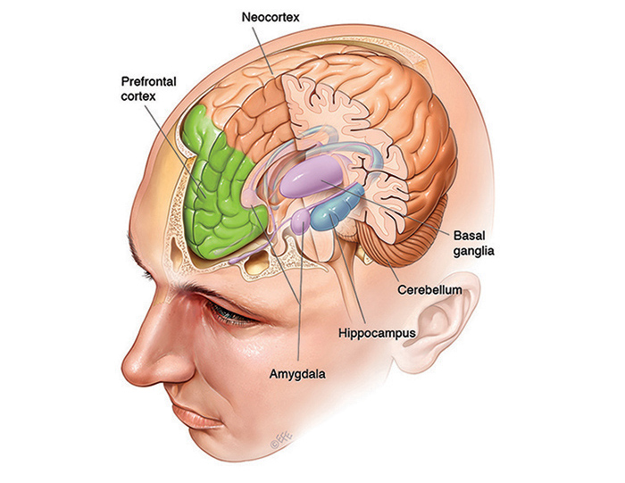
The Cerebellum: Expansion as Precision

The cerebellum contains roughly 80% of the brain’s neurons, the vast majority of which are granule cells [8]. Its input arrives via mossy fibres as a relatively low-dimensional signal — motor states, sensory feedback, contextual cues. The cerebellum immediately explodes this into an enormous population of granule cell activations: the input is mapped into a space of order \(10^{10}\) or more dimensions, with extremely sparse activation (only a tiny fraction of granule cells active at any moment).

What does this buy? Pattern separation. Two motor commands that are nearly identical in low-dimensional space — “move my arm 10 degrees” and “move my arm 11 degrees” — will, after expansion into the granule cell layer, activate largely non-overlapping populations. They become, in Cover’s theorem’s language, linearly separable. The Purkinje cells that read out from the granule layer can learn to discriminate them with a simple linear threshold.

This is expansion coding: the cerebellum is implementing, in neural hardware, exactly what kernel methods implement mathematically. It is mapping inputs into a space where linear readout suffices, using sparse random-like projections that preserve the geometry of the input manifold while making fine distinctions tractable.

The price is that nothing generalises at the granule cell level. Every new context activates a new, essentially orthogonal pattern. The cerebellum is not in the business of abstraction; it is in the business of precision.

The Neocortex: Compression as Generalisation

The neocortex operates as a hierarchical compression engine [9]. The canonical example is the ventral visual stream — the pathway from primary visual cortex (V1) to inferotemporal cortex (IT) that underlies object recognition.

Raw retinal input is high-dimensional: millions of photoreceptors encoding pixel-level light intensities. As signals propagate up the hierarchy, successive areas discard information that is irrelevant to object identity — exact pixel positions, local contrast, low-level edge orientations — and preserve information that is invariant across viewing conditions: object shape, part configuration, surface texture. By the time the representation reaches IT cortex, a face is represented by a low-dimensional pattern that fires consistently regardless of whether the face is seen from the left, the right, in bright light, or in shadow [10].

This is manifold compression: the neocortex is learning the intrinsic low-dimensional manifold of object identity, stripping away the high-dimensional variation that is due to viewing conditions rather than object properties. The result is a representation that generalises beautifully — you recognise a friend’s face under any lighting condition — but that cannot distinguish fine-grained details when they are critical.

The Hippocampus: Both at Once

The hippocampus is where the two strategies meet, and its internal architecture is a microcosm of the full expansion-compression story [11].

• The dentate gyrus (DG) performs extreme expansion: approximately \(10^6\) granule cells receive input from roughly \(10^7\) entorhinal cortex neurons, with very sparse coding (~5% active). Each episode, each memory, is mapped to a largely orthogonal high-dimensional pattern. This is pattern separation at its most extreme — the reason you can distinguish this morning’s breakfast from yesterday’s, despite them sharing almost all features.

• CA3 uses dense recurrent connectivity to perform pattern completion: given a partial or degraded input, it reconstructs the full stored pattern. This is the manifold-like operation — it maps the noisy partial input onto the nearest attractor in a learned landscape of stored memories.

• CA1 then compresses back to a compact index, integrating the CA3 completion with direct entorhinal input to form a final contextual representation.

The hippocampal circuit is, in essence, a learned compressor-expander: it stores experiences by first separating them (DG), enabling recall from partial cues (CA3), and then indexing them efficiently (CA1). The same circuit that enables you to recall yesterday’s lunch in full detail from a single smell is also what enables you to generalise “lunch” as a concept across all instances.

Why Machine Learning Needs Both

Current deep learning models are, structurally, predominantly neocortical: they are compression engines. A ResNet, a Vision Transformer, a large language model — all of these are hierarchical compression machines that learn to map high-dimensional input onto low-dimensional manifolds. They generalise admirably. They fail at precise discrimination when fine-grained distinctions matter, and they struggle to bind features into structured compositional wholes.

The cerebellar strategy — high-dimensional sparse expansion for discriminability — appears in machine learning mainly as a historical artefact (the kernel trick, radial basis function networks) or as a computational trick (random feature methods, locality-sensitive hashing). It has not been deeply integrated into the representational philosophy of modern architectures.

What is almost entirely absent is the loop: the closed circuit between expansion and compression, the feedback that allows the brain to use discrimination to sharpen generalisation and generalisation to guide discrimination. The thalamus, basal ganglia, and dopaminergic modulation systems implement this loop biologically. Machine learning has gradient descent, which is a crude approximation — but it operates on the full network simultaneously rather than as a structured interplay between specialised subsystems.

---

Part III: Vector Symbolic Architectures — Algebra in a High-Dimensional Space

The Core Idea

Vector Symbolic Architectures (VSAs) [12, 13] are a family of frameworks that address a different gap: not the expansion-compression trade-off, but the question of compositional structure. How do you represent the fact that “the red ball is to the left of the blue cube” in a way that supports inference, binding, and decomposition?

The standard neural network answer is: learn it from data, hope the structure is implicit in the weights. The VSA answer is: use mathematics. Encode all atomic concepts as random high-dimensional vectors, and use algebraic operations — binding, superposition, permutation — to compose them into structured representations.

The key insight, which is the bridge between Cover’s theorem and distributed representation, is this: in a sufficiently high-dimensional space, random vectors are approximately orthogonal to each other. If you draw two random unit vectors in \(\mathbb{R}^d\), their expected inner product is 0, with standard deviation \(1/\sqrt{d}\). In \(d = 10000\), the expected angle between two random vectors is within \(0.6°\) of 90°. This means that a high-dimensional space can hold an exponentially large number of “symbols” — random vectors — that are all approximately orthogonal, and therefore approximately non-interfering.

VSAs exploit this property to build a kind of distributed algebra: you can add, multiply, and permute high-dimensional vectors to encode structured information, and the result is a single high-dimensional vector — no bigger than the originals — that can be queried to recover the components. A reference YouTube video for explanation

The Major VSA Families

Holographic Reduced Representations (HRR) [12]: Real-valued vectors of fixed dimension \(d\). Binding is circular convolution:

\[\mathbf{a} \circledast \mathbf{b} = \text{IFFT}(\text{FFT}(\mathbf{a}) \cdot \text{FFT}(\mathbf{b}))\]

Superposition is vector addition. Unbinding is approximate (circular correlation with the approximate inverse). HRRs can represent nested structures — “(colour:red) + (shape:sphere) + (position:left)” as a single vector — and partially recover components via querying. The connection to the Fourier domain is not incidental: circular convolution is element-wise multiplication in frequency space, making HRRs a natural signal-processing object.

Binary Spatter Codes (BSC) [14]: Binary vectors \(\{0,1\}^d\). Binding is XOR, superposition is majority vote. Extremely hardware-efficient — binding is a single bitwise operation — and well-suited to neuromorphic or edge computing. The binary constraint limits capacity and expressiveness compared to real or complex variants.

MAP-C (Multiply-Add-Permute, Complex) [15]: Phasor vectors on the unit circle in \(\mathbb{C}^d\) — each component has magnitude 1 and a phase \(\theta \in [0, 2\pi)\). Binding is element-wise complex multiplication (phase addition):

\[(\mathbf{a} \otimes \mathbf{b})_i = a_i \cdot b_i = e^{i(\theta_i^a + \theta_i^b)}\]

Superposition is vector summation. Crucially, unbinding is exact: the inverse of complex multiplication is conjugation, \((\mathbf{a} \otimes \mathbf{b}) \otimes \bar{\mathbf{a}} = \mathbf{b}\). MAP-C has the highest known capacity for clean symbolic algebra in VSAs and is currently state-of-the-art for lossless compositional structure.

Fourier HRR (FHRR) [16]: Equivalent to MAP-C but framed explicitly in terms of the Discrete Fourier Transform. Binding in FHRR is multiplication in the frequency domain — which is convolution in the time domain. This framing makes the connection to signal processing fully explicit: FHRR is HRR where the carrier is the Fourier basis, and binding corresponds to phase-shift convolution. This is why FHRR representations are particularly natural for encoding temporal or spectral structure.

Resonator Networks [17]: Not a VSA variant but a VSA algorithm. Given a product vector \(\mathbf{z} = \mathbf{a} \otimes \mathbf{b} \otimes \mathbf{c}\), how do you recover \(\mathbf{a}\), \(\mathbf{b}\), and \(\mathbf{c}\) without brute-force search? Resonator networks solve this via a recurrent attractor dynamic: start with noisy estimates of each factor, iteratively update each estimate using the others, and converge to the true factors. The name comes from the resonance-like dynamics — factors “lock in” when they become mutually consistent. This is analogous to phase-locking in neural oscillator networks.

Sparse Distributed Memory (SDM) [14]: Kanerva’s foundational framework, predating the formal VSA literature. A content-addressable memory over a very high-dimensional binary address space, where reading and writing are distributed across all addresses within a Hamming-distance threshold. SDM is closely related to the Hopfield network in its attractor dynamics, and to the hippocampal CA3 pattern completion system. It is not strictly a VSA but shares the philosophy of distributed, superposed representation.

Binding and Superposition as Neural Operations

The two core VSA operations have direct neural correlates:

Superposition (vector addition) corresponds to the summation of neural activity across populations. If the population code for concept A is a pattern of firing rates, and for concept B is another pattern, then the simultaneous activation of both produces the superposition. The brain routinely maintains superposed representations — this is the mechanism behind working memory, where multiple items are held simultaneously without being confused, via slight phase offsets or temporal multiplexing.

Binding (circular convolution or complex multiplication) corresponds to temporal synchronisation or oscillatory coupling. The binding problem in neuroscience [18] asks: when you see a red ball and a blue cube simultaneously, how does the brain keep “red” bound to “ball” and “blue” bound to “cube,” rather than mixing them into “red cube” and “blue ball”? The dominant hypothesis is that features of the same object oscillate at the same phase in the gamma band (~40 Hz), while features of different objects oscillate at different phases. Phase is the binding operator in the brain, just as complex multiplication is the binding operator in MAP-C and FHRR.

This parallel is deep and not accidental. FHRR/MAP-C, with its unit-circle phasors and phase-addition binding, is a direct mathematical model of the phase-coding hypothesis of neural binding. The fact that this gives the highest VSA capacity is not surprising: the brain has been optimising this architecture for hundreds of millions of years.

---

Part IV: Distributed Representations and Multimodal Generalisation

Why Point Representations Fail at Multimodality

The standard approach to multimodal learning is: train modality-specific encoders, project their outputs into a shared \(\mathbb{R}^d\), and train contrastive or generative objectives to align the resulting points [19]. A cat image and a spoken description of a cat should land near the same point. This works remarkably well within modalities and for cross-modal retrieval.

But it fails at genuine compositional multimodal reasoning — the kind of task that requires understanding the structure of a scene, not just its identity. “Is the object to the left of the red thing also blue?” requires binding spatial relations, object identities, and colour attributes into a structured representation that can be queried compositionally. A point in \(\mathbb{R}^d\) encodes none of that structure explicitly; it is a holistic summary that has thrown away the compositional information.

VSAs provide exactly the structure that is missing. Consider encoding a simple visual scene with two objects:

\[\mathbf{scene} = (\mathbf{colour\_red} \otimes \mathbf{shape\_ball} \otimes \mathbf{pos\_left}) + (\mathbf{colour\_blue} \otimes \mathbf{shape\_cube} \otimes \mathbf{pos\_right})\]

This is a single vector in \(\mathbb{R}^d\) (or \(\mathbb{C}^d\)). But it supports structured queries:

\[\mathbf{scene} \otimes \mathbf{pos\_left}^{-1} \approx \mathbf{colour\_red} \otimes \mathbf{shape\_ball}\]

You can ask “what is at the left position?” by binding with the inverse of the position vector and reading out the approximate match from a codebook. This is compositional inference, performed by algebraic operations on distributed representations — no symbolic reasoner required, no explicit graph traversal.

The Expansion-VSA Connection

Here the two threads of this blog meet. Cover’s theorem says that high-dimensional spaces make patterns linearly separable. VSAs say that high-dimensional spaces can hold exponentially many approximately orthogonal symbols. These are two expressions of the same underlying geometry.

The cerebellum’s expansion coding and VSA superposition are both exploiting the same high-dimensional geometry: the fact that random vectors in \(\mathbb{R}^d\) are approximately orthogonal, and that therefore you can pack many non-interfering patterns into the same space. The difference is:

• Cerebellum: the high-dimensional space is used for discrimination — to separate similar patterns so that fine-grained readout is possible. The structure is sparse and approximately random.
• VSA: the high-dimensional space is used for composition — to bind structured relationships into a single vector that can be algebraically decomposed. The structure is algebraically organised.

A full neural architecture that takes inspiration from both would: 1. Expand multimodal inputs into high-dimensional sparse representations for discrimination (cerebellar strategy) 2. Bind feature representations into structured compositional vectors using VSA operations (algebraic strategy) 3. Compress the composed representations onto a low-dimensional manifold for generalisation (neocortical strategy) 4. Close the loop with feedback that uses generalisation to guide expansion and discrimination to refine composition

This is not a hypothetical future architecture. All of these components exist, in some form, in the current ML literature. What is missing is their integration into a coherent representational framework.

What Else Is Out There

The VSA landscape is not the only set of distributed representation tools worth knowing. Several other formalisms address adjacent problems:

Tensor Networks (Matrix Product States, MERA) [20] come from quantum physics and represent high-order joint distributions as networks of low-rank tensor contractions. They are powerful for data with strong local structure — sequences, grids — and map naturally onto the structure of attention in Transformers. For signal data with spectral structure, tensor trains (TT-decompositions) can represent complex multi-dimensional tensors with far fewer parameters.

Geometric / Clifford Algebra [21] generalises complex numbers, quaternions, and exterior algebra into a single framework where vectors, bivectors, and multivectors compose via the geometric product. For data with intrinsic geometric structure — 3D rotations, electromagnetic fields, physical simulations — Clifford algebra representations are equivariant by construction. They are underexplored in ML relative to their mathematical power.

Scattering Transforms [22] are wavelet-based, non-learned feature extractors that are provably stable under small deformations of the input. They extract hierarchical frequency information without any learning, and are particularly well-suited to non-stationary signals (audio, EEG, seismic data). For signal modalities where stability matters more than reconstruction, scattering transforms provide a principled alternative to learned encoders.

Sparse Coding / Dictionary Learning [23] decomposes signals as sparse linear combinations of learned basis atoms. This is philosophically different from VSA — there is no symbolic binding — but it is among the best methods for raw signal representation, and its atoms can be interpreted as the elementary features that the model has learned to recognise.

---

The Picture That Emerges

Let me close with the picture that the two blogs in this series are collectively building.

High-dimensional spaces are, in a precise sense, more linear: Cover’s theorem and Johnson-Lindenstrauss tell us that classification problems become separable and geometric structure is preserved under random projection. The brain’s cerebellar expansion exploits this geometry for discrimination. VSAs exploit it for compositional algebra.

Low-dimensional spaces are curved: the Manifold Hypothesis tells us that real data occupies a low-dimensional manifold with intrinsic curvature, and representing that manifold in a flat coordinate system requires nonlinear maps. The neocortex’s hierarchical compression exploits this structure for generalisation. Modern deep learning is, largely, an implementation of this strategy.

The brain does both, in a specific circuit with feedback loops. Current ML does predominantly the second. The gap is felt most acutely in multimodal reasoning, where you need to generalise across modalities (neocortical compression) while maintaining compositional structure (VSA algebra) and fine-grained discriminability (cerebellar expansion).

The next step — for the field, and for this series — is to ask whether VSAs, signals, and manifold theory can be integrated into a single framework. In particular: can a VSA with complex phasor vectors, whose binding operation is phase multiplication and whose superposition is signal summation, be understood as a representation in a Hilbert function space? Can the resonator network’s attractor dynamics be related to the hippocampus’s pattern completion? Can the expansion-compression loop be implemented differentiably?

These are open questions. But the mathematical vocabulary to ask them precisely now exists.

---

References

[1] Cover, T. M. (1965). Geometrical and statistical properties of systems of linear inequalities with applications in pattern recognition. IEEE Transactions on Electronic Computers, EC-14(3), 326–334.

[2] Schölkopf, B., & Smola, A. J. (2002). Learning with Kernels: Support Vector Machines, Regularization, Optimization, and Beyond. MIT Press.

[3] Johnson, W. B., & Lindenstrauss, J. (1984). Extensions of Lipschitz mappings into a Hilbert space. Contemporary Mathematics, 26, 189–206.

[4] Fefferman, C., Mitter, S., & Narayanan, H. (2016). Testing the manifold hypothesis. Journal of the American Mathematical Society, 29(4), 983–1049.

[5] Brahma, P. P., Wu, D., & She, Y. (2016). Why deep learning works: A manifold disentanglement perspective. IEEE Transactions on Neural Networks and Learning Systems, 27(10), 1997–2008.

[6] Cabannes, V., Bottou, L., & Balestriero, R. (2023). Ssl back to basics: Addressing practical challenges in self-supervised learning. arXiv:2304.09438.

[7] Marr, D. (1969). A theory of cerebellar cortex. Journal of Physiology, 202(2), 437–470.

[8] Ito, M. (2008). Control of mental activities by internal models in the cerebellum. Nature Reviews Neuroscience, 9(4), 304–313.

[9] DiCarlo, J. J., Zoccolan, D., & Rust, N. C. (2012). How does the brain solve visual object recognition? Neuron, 73(3), 415–434.

[10] Tanaka, K. (1996). Inferotemporal cortex and object vision. Annual Review of Neuroscience, 19(1), 109–139.

[11] O’Reilly, R. C., & McClelland, J. L. (1994). Hippocampal conjunctive encoding, storage, and recall: avoiding a trade-off. Hippocampus, 4(6), 661–682.

[12] Plate, T. A. (1995). Holographic reduced representations. IEEE Transactions on Neural Networks, 6(3), 623–641.

[13] Kanerva, P. (2009). Hyperdimensional computing: An introduction to computing in distributed representation with high-dimensional random vectors. Cognitive Computation, 1(2), 139–159.

[14] Kanerva, P. (1988). Sparse Distributed Memory. MIT Press.

[15] Gayler, R. W. (2004). Vector symbolic architectures answer Jackendoff’s challenges for cognitive neuroscience. arXiv:cs/0412059.

[16] Plate, T. A. (2003). Holographic Reduced Representations: Distributed Representation for Cognitive Structures. CSLI Publications.

[17] Frady, E. P., Kent, S. J., Olshausen, B. A., & Sommer, F. T. (2020). Resonator networks, 1: An efficient solution for factoring high-dimensional, distributed representations of data structures. Neural Computation, 32(12), 2311–2331.

[18] Singer, W. (1999). Neuronal synchrony: A versatile code for the definition of relations? Neuron, 24(1), 49–65.

[19] Radford, A., et al. (2021). Learning transferable visual models from natural language supervision (CLIP). ICML 2021. https://arxiv.org/abs/2103.00020

[20] Stoudenmire, E. M., & Schwab, D. J. (2016). Supervised learning with tensor networks. NeurIPS 2016. https://arxiv.org/abs/1605.05775

[21] Ruhe, D., Gupta, J. K., de Boer, S., Brandstetter, J., & Forré, P. (2023). Clifford neural layers for PDE modeling. ICLR 2023. https://arxiv.org/abs/2209.04934

[22] Mallat, S. (2012). Group invariant scattering. Communications on Pure and Applied Mathematics, 65(10), 1331–1398.

[23] Olshausen, B. A., & Field, D. J. (1996). Emergence of simple-cell receptive field properties by learning a sparse code for natural images. Nature, 381(6583), 607–609.

---

Blog 3 of this series will go deeper into Vector Symbolic Architectures as signal representations: why MAP-C/FHRR phasor vectors are natural elements of a Hilbert function space, how Resonator Networks relate to hippocampal pattern completion, and what a differentiable expansion-compression loop might look like as a neural architecture.

---

Tags: distributed-representations vector-symbolic-architectures manifold-hypothesis neuroscience multimodal-learning hyperdimensional-computing compositional-reasoning machine-learning

Topological Spaces

From Points to Waves: Why the Next Generation of AI Representations Should Think in Signals

Blog 1 of a series on Topology, and the Future of Machine Learning Representation

---

“A vector tells you where something is. A signal tells you what something does.”

---

A Personal Starting Point

Over the past year, I have been working on problems that sit at the intersection of signals and cognition — including sleep-stage classification, cognitive performance modelling, and participation in the EEG 2025 NeurIPS challenge. These experiences exposed me to biological signals not just as data, but as structured, dynamic processes: oscillations, rhythms, synchrony, and noise interacting over time.

This naturally led me to think about representation from a more neuroscientific perspective. In the brain, information is not encoded as static points — it is carried through patterns of activity, often oscillatory, where timing and phase relationships play a crucial role. That raised a simple but persistent question:

Why do we represent meaning in machine learning as a static point in space?

Language is not static. Images are not static. The world that machine learning models are trying to understand is fundamentally dynamic — things unfold, interact, interfere with each other, and change meaning depending on context and timing. And yet the dominant paradigm in representation learning is to compress all of that into a fixed vector: a point in \(\mathbb{R}^d\) that just sits there.

I started thinking about what it would look like to represent multimodal data — text, audio, vision — not as vectors but as signals: functions over time or frequency, things that have phase as well as amplitude, things that can constructively amplify each other or destructively cancel. Then I discovered that a whole family of models — State Space Models, including S4 [1] and Mamba [2] — had already begun moving in this direction, using signal-processing machinery from control theory as the foundation of sequence modelling.

This blog series is an attempt to explore an alternative viewpoint: what if representations were not points, but signals? I am writing this series to document my learning from first principles and to make that journey useful to others exploring similar questions. I have also used LLMs for ideation, restructuring, and rephrasing in places, but the core ideas, technical direction, and learning are my own. The mathematical equations explaining each of the spaces are also generated using LLMs.

Let us begin with the spaces themselves.

---

Part I: The Hierarchy of Mathematical Spaces

Before we can argue that one kind of space is better for representation, we need to understand what a “space” actually is in mathematics, and what properties different spaces add on top of each other. Think of this as a ladder — each rung adds structure. Watch the reference video

Hierarchy of Mathematical Spaces

Image source: reference image

1. Topological Space — The Most General Setting

A topological space is the most general notion of a geometric space. [3]. You start with a set \(X\) and a collection of subsets called open sets, satisfying three axioms: the empty set and \(X\) itself are open; arbitrary unions of open sets are open; finite intersections of open sets are open.

That is all. There is no notion of distance, no notion of angle, no notion of size. But you gain the concept of continuity — a map between two topological spaces is continuous if the preimage of every open set is open.

This matters for machine learning because continuity is the prerequisite for anything meaningful to happen. If your embedding function is not continuous, nearby inputs can map to wildly different representations, and generalisation becomes impossible. Topological spaces are the setting where we ask: what structure must be preserved when we learn a mapping?

2. Metric Space — Adding Distance

A metric space \((X, d)\) is a topological space equipped with a distance function \(d : X \times X \to \mathbb{R}_{\geq 0}\) satisfying non-negativity, identity of indiscernibles (\(d(x,y) = 0 \iff x = y\)), symmetry, and the triangle inequality \(d(x,z) \leq d(x,y) + d(y,z)\) [4].

Metric spaces are where most practising ML researchers implicitly live. Euclidean distance, cosine distance, edit distance — these are all metrics. The key concept metric spaces give us is convergence: a sequence \(\{x_n\}\) converges to \(x\) if \(d(x_n, x) \to 0\).

But metric spaces say nothing about directions, addition, or scaling. Two points have a distance between them, but you cannot add them together and get something meaningful.

3. Normed Vector Space — Adding Size and Algebra

A normed vector space \((V, \|\cdot\|)\) is a vector space over \(\mathbb{R}\) (or \(\mathbb{C}\)) equipped with a norm \(\|\cdot\| : V \to \mathbb{R}_{\geq 0}\) satisfying positive definiteness, absolute homogeneity (\(\|\alpha v\| = |\alpha| \|v\|\)), and the triangle inequality [4].

Every normed vector space is a metric space under \(d(x,y) = \|x - y\|\). But now we can also add vectors and scale them, which means we can talk about linear combinations, subspaces, and transformations.

This is where the \(L^p\) spaces live. \(L^2(\Omega)\) — the space of square-integrable functions on a domain \(\Omega\) — is a normed vector space with \(\|f\|_2 = \left(\int_\Omega |f(x)|^2 \, dx\right)^{1/2}\). This is deeply relevant: signals with finite energy (finite \(L^2\) norm) form a normed vector space, and this is the foundation of all of Fourier analysis.

4. Inner Product Space — Adding Geometry and Angles

An inner product space adds a bilinear (or sesquilinear, over \(\mathbb{C}\)) form \(\langle \cdot, \cdot \rangle : V \times V \to \mathbb{F}\) satisfying conjugate symmetry, linearity in the first argument, and positive definiteness [3].

The norm is recovered as \(\|v\| = \sqrt{\langle v, v \rangle}\). But crucially, the inner product adds angles:

\[\cos\theta = \frac{\langle u, v \rangle}{\|u\| \|v\|}\]

This is the space that current LLMs inhabit. Dot-product attention computes \(\text{Attention}(Q, K) \propto QK^\top\), which is exactly a matrix of inner products [5]. Cosine similarity, used ubiquitously for semantic search, measures the angle between embedding vectors. The geometry of meaning, in today’s models, is entirely encoded in the angles and magnitudes of vectors in an inner product space.

5. Banach Space — Completeness

A Banach space is a normed vector space that is complete: every Cauchy sequence converges to a limit that is still inside the space [4]. This is a technical but important property. Incompleteness means you can construct sequences of valid representations that “converge” to something outside your representation space — a pathological situation for any learning algorithm.

All finite-dimensional normed vector spaces are automatically Banach spaces. For infinite-dimensional function spaces (which appear in functional analysis and in the theory of neural networks as models of function classes), completeness must be verified explicitly.

6. Hilbert Space — The Meeting Point of Algebra and Analysis

A Hilbert space \(\mathcal{H}\) is a complete inner product space [3,4]. It combines the geometric richness of an inner product space with the analytical solidity of a Banach space. In finite dimensions, this is nothing new — \(\mathbb{R}^d\) with the dot product is already a Hilbert space.

The profound content of Hilbert spaces appears in infinite dimensions. The canonical example is \(L^2(\mathbb{R})\): the space of square-integrable functions on the real line. This space has:

• An inner product: \(\langle f, g \rangle = \int_{-\infty}^\infty f(x)\overline{g(x)} \, dx\)
• A notion of orthogonality: \(\langle f, g \rangle = 0\)
• Orthonormal bases: the complex exponentials \(\{e^{2\pi i n x}\}_{n \in \mathbb{Z}}\) form an orthonormal basis — this is the Fourier basis
• A Plancherel theorem: the Fourier transform is an isometric isomorphism on \(L^2(\mathbb{R})\), preserving inner products exactly

This last point is crucial: the Fourier transform is a rotation in Hilbert space. Moving from the time domain to the frequency domain is not a loss of information — it is a change of basis in an infinite-dimensional inner product space.

7. Other Spaces

Sobolev spaces extend function spaces by incorporating derivatives. [6]. They are the natural setting for partial differential equations and for understanding the regularity of functions — not just whether they are square-integrable, but whether they are smooth.

In machine learning, Sobolev spaces appear in regularisation theory (penalising functions with large higher-order derivatives), in physics-informed neural networks, and in the theoretical analysis of approximation by neural networks with smooth activation functions [7].

Minkowski space introduces an indefinite inner product.

This is the geometric setting of special relativity. In machine learning, it appears in hyperbolic embedding methods [9]: because hyperbolic space has constant negative curvature, it can represent hierarchical structures (trees, taxonomies, knowledge graphs) exponentially more efficiently than Euclidean space. The Poincaré ball model of hyperbolic space can be viewed as a projection of Minkowski space.

---

Part II: What LLMs Are Actually Doing — and What They Are Missing

Embeddings as Static Vectors

In every major large language model — GPT-4 [10], Llama [11], Mistral — words and subword tokens are mapped to vectors in \(\mathbb{R}^d\) for some large \(d\) (commonly 1024 to 16384). These embeddings are static: the token “bank” always starts as the same point in \(\mathbb{R}^d\), regardless of context. Context-sensitivity comes later, through the attention mechanism, which produces contextualised representations by mixing embeddings.

The geometry of these spaces is straightforward:

• Semantic similarity is measured by cosine similarity (angle in the inner product space)
• Attention scores are inner products, \(q^\top k / \sqrt{d_k}\), softmax-normalised [5]
• Residual connections perform vector addition in the same space

This is a rich geometric structure, and it has proven extraordinarily effective. But it has a fundamental character: it is amplitude-only. Every representation is a real-valued vector — a collection of magnitudes. There is no phase, no timing information, no notion of whether two features are in sync or in opposition.

The Magnitude Heuristic and Its Failure Modes

In real-valued networks, the common heuristic is: a feature is important if its activation is large. Magnitude proxies for salience. This creates several problems:

1. Frequency vs importance ambiguity: A feature that fires frequently in training data accumulates large weights, making it hard to distinguish structural relevance from statistical prevalence.
2. Superposition: Polysemantic neurons — single neurons that respond to multiple unrelated concepts — have been extensively documented [12]. When you only have magnitude, many concepts must be packed into the same activation by sharing magnitude ranges.
3. Limited interaction mechanisms: In real-valued spaces, you cannot have two representations that destructively interfere. The only way to suppress a feature is to add a neuron with the opposite sign — which uses capacity but does not reflect any geometric elegance.

Hardy Spaces and the Frequency Domain View

The Laplace transform maps a continuous-time signal \(f(t)\) to a function of a complex variable \(s = \sigma + i\omega\):

\[\mathcal{L}\{f\}(s) = \int_0^\infty f(t) e^{-st} \, dt\]

The Z-transform does the same for discrete sequences:

\[\mathcal{Z}\{x\}(z) = \sum_{n=0}^\infty x[n] z^{-n}\]

The spaces of functions that these transforms naturally live in are Hardy spaces \(H^2\) — a class of Hilbert spaces consisting of holomorphic (complex-analytic) functions on a half-plane or disk, with \(L^2\) boundary behaviour [13]. Hardy spaces inherit the inner product structure of \(L^2\), but the analyticity constraint (the real and imaginary parts satisfy the Cauchy-Riemann equations) means they encode much more structure than generic \(L^2\) functions.

In these spaces, a “signal” is not a point but a function: a complex-valued object where:

• The real part encodes amplitude information
• The imaginary part encodes phase information
• The inner product measures overlap, synchrony, and coherence between signals

This is the geometric framework that has been standard in electrical engineering and quantum mechanics for decades, but is only beginning to enter machine learning in earnest.

---

Part III: Signals as Richer Representations

Complex Activations and Phase

In a complex-valued neural network (CVNN) [14], activations are elements of \(\mathbb{C}\) rather than \(\mathbb{R}\). A single complex activation \(z = re^{i\theta}\) encodes two quantities:

• \(r = |z|\): the magnitude (analogous to standard activation strength)
• \(\theta = \arg(z)\): the phase (a second, independent channel of information)

Phase encodes relational information — not “how strong is this feature?” but “how does this feature relate to the system’s current state?” This is the representation language of physical systems: waves in quantum mechanics, oscillators in neuroscience, carrier signals in communications.

Interference: The Mechanism That Real-Valued Networks Lack

The defining operation of wave-based representations is interference. When two complex-valued signals are summed:

\[z_1 + z_2 = r_1 e^{i\theta_1} + r_2 e^{i\theta_2}\]

the result depends critically on the phase relationship \(\theta_1 - \theta_2\):

• If \(\theta_1 = \theta_2\) (in phase): constructive interference — amplitudes add
• If \(\theta_1 = \theta_2 + \pi\) (out of phase): destructive interference — amplitudes cancel
• Intermediate phases: partial interference of intermediate strength

This gives a principled mechanism for:

1. Noise suppression: Stochastic noise has a uniform phase distribution. When many noisy signals are summed, their phases cancel in expectation — this is exactly how phase-array radar and optical coherence tomography work [15]. Real-valued networks have no analogous mechanism.

2. Feature synchronisation: Semantically related features can be “phase-locked” — assigned similar phases so they constructively amplify each other. This is reminiscent of the binding hypothesis in neuroscience [16]: objects are perceived as unified wholes because their neural representations oscillate in phase.

3. Geometric stability: Phase-aware models encode relationships as rotations in the complex plane, not just as signed magnitudes. Rotations are isometries — they preserve distances — which tends to improve generalisation and reduce sensitivity to input perturbations.

Why This Matters for Multimodal Representations

My original motivation was multimodal representation: representing text, image, and audio in a common space. The standard approach is to train modality-specific encoders and project them into the same \(\mathbb{R}^d\) — forcing fundamentally different signal types into the same geometric box.

But audio is intrinsically a signal: it is a pressure wave with frequency, amplitude, and phase. Representing audio as a static point in \(\mathbb{R}^d\) discards its temporal structure before the representation even begins. A Hilbert space representation would allow audio, image (via 2D Fourier structure), and text (via sequence dynamics) to be represented as functions — elements of an \(L^2\) space — and their cross-modal relationships to be encoded as inner products and phase relationships in that space.

---

Part IV: State Space Models — The Existing Bridge

When I was developing these ideas, I came across a body of work that had already built something close to what I was imagining, coming from a different direction: State Space Models (SSMs).

The S4 model [1] parameterises sequence processing using a continuous-time state space:

\[\dot{x}(t) = Ax(t) + Bu(t), \quad y(t) = Cx(t) + Du(t)\]

where \(A\) is a structured matrix (specifically, a HiPPO matrix [17] designed to optimally memorise history), and the model is discretised for practical training. The key insight: in the frequency domain (via Laplace transform), this system is a rational function of \(s\) — exactly the kind of object that lives naturally in a Hardy space.

Mamba [2] extends this with selective state spaces — input-dependent dynamics that allow the model to choose, at each step, what to remember and what to forget. This is closer to a filter in signal processing than to attention: rather than computing pairwise similarities across the entire sequence, it propagates information through a dynamical system with state.

The computational advantage is stark: standard Transformers scale as \(O(n^2)\) in sequence length due to the attention matrix, while SSMs scale as \(O(n)\) — because they process sequences as signals through a filter, not as sets of points comparing each other.

This is not a coincidence. When you represent sequences as signals rather than as sets, linear-time processing becomes natural. The Fourier transform of a signal is computed in \(O(n \log n)\) rather than \(O(n^2)\); convolution in the time domain is multiplication in the frequency domain. Signal representations come with efficient algorithms as a structural gift.

---

Part V: A Taxonomy of Spaces for Representation

To ground the above discussion, here is a summary of which spaces are relevant to which ML contexts:

Space	Key Structure	Natural ML Application
Metric space	Distance only	k-NN, clustering, contrastive learning
Normed vector space	Distance + linear algebra	\(L^p\) regularisation, weight decay
Inner product space	Angles + projections	Dot-product attention, cosine similarity
Hilbert space (finite-dim)	Complete inner product	Standard neural network layers
Hilbert space (infinite-dim, \(L^2\))	Function-valued representations	SSMs, functional neural processes
Hardy space \(H^2\)	Holomorphic + \(L^2\) boundary	Laplace/Z-transform signal representations
Sobolev space \(W^{k,p}\)	Function + derivative regularity	Physics-informed NNs, smoothness regularisation
Hyperbolic space / Minkowski	Negative curvature	Hierarchical embedding, knowledge graphs
Riemannian manifold	Local Euclidean + curvature	Geometric deep learning, manifold learning

The progression from left to right is a progression from less structure to more structure. Current LLMs sit solidly in the finite-dimensional inner product space column. State space models begin to occupy the \(L^2\) and Hardy space columns. The full realisation of signal-based multimodal representation would require working fluently across several of these spaces simultaneously.

---

Conclusion: Rethinking Representation from the Ground Up

The dominant paradigm treats representation as placement: a token is a point, a meaning is a location, similarity is proximity. This is a powerful and productive view, and it has driven remarkable progress. But it is, ultimately, a static view.

Signals offer a dynamic alternative. A representation that carries phase as well as amplitude can encode how a feature relates to the system’s current state, not just that it is present. Representations as functions in a Hilbert space can encode temporal and spectral structure natively, without discarding it at the tokenisation stage. Interference gives a principled mechanism for noise suppression and feature binding that has no real-valued analogue.

State space models are an existence proof that this direction is practically viable. But I think the full potential — particularly for multimodal systems where audio, vision, and language need to be represented in a common framework that respects the intrinsic nature of each modality — remains largely unexplored.

The next blog in this series will move from spaces to geometry: we will look at the Manifold Hypothesis and ask what it means for data to live on a low-dimensional manifold inside a high-dimensional space, explore whether high-dimensional spaces are really “more linear” in any meaningful sense, and introduce Vector Symbolic Architectures as a way to perform structured reasoning inside geometric spaces.

---

References

[1] Gu, A., Goel, K., & Ré, C. (2022). Efficiently modeling long sequences with structured state spaces. ICLR 2022. arXiv

[2] Gu, A., & Dao, T. (2023). Mamba: Linear-time sequence modeling with selective state spaces. arXiv:2312.00752. arXiv

[3] Reed, M., & Simon, B. (1980). Methods of Modern Mathematical Physics, Vol. 1: Functional Analysis. Academic Press.

[4] Kreyszig, E. (1978). Introductory Functional Analysis with Applications. Wiley.

[5] Vaswani, A., et al. (2017). Attention is all you need. NeurIPS 2017. arXiv

[6] Evans, L. C. (2010). Partial Differential Equations (2nd ed.). American Mathematical Society.

[7] Barron, A. R. (1993). Universal approximation bounds for superpositions of a sigmoidal function. IEEE Transactions on Information Theory, 39(3), 930–945.

[8] Minkowski, H. (1908). Raum und Zeit. Physikalische Zeitschrift, 10, 75–88.

[9] Nickel, M., & Kiela, D. (2017). Poincaré embeddings for learning hierarchical representations. NeurIPS 2017. arXiv

[10] OpenAI. (2023). GPT-4 Technical Report. arXiv:2303.08774. arXiv

[11] Touvron, H., et al. (2023). LLaMA: Open and efficient foundation language models. arXiv:2302.13971. arXiv

[12] Elhage, N., et al. (2022). Toy models of superposition. Transformer Circuits Thread. Article

[13] Garnett, J. B. (2007). Bounded Analytic Functions. Springer.

[14] Trabelsi, C., et al. (2018). Deep complex networks. ICLR 2018. arXiv

[15] Trees, H. L. V. (2002). Optimum Array Processing. Wiley-Interscience.

[16] Singer, W. (1999). Neuronal synchrony: a versatile code for the definition of relations? Neuron, 24(1), 49–65.

[17] Gu, A., et al. (2020). HiPPO: Recurrent memory with optimal polynomial projections. NeurIPS 2020. arXiv

---

This is Blog 1 of a planned series. Blog 2 will cover the Manifold Hypothesis, the question of linearity in high-dimensional spaces, and Vector Symbolic Architectures as a framework for compositional reasoning inside geometric representations.

---

Tags: representation-learning hilbert-spaces state-space-models signal-processing machine-learning mathematical-foundations embeddings

Simple Battleship game using Python

To run this code, one must have NumPy and Pandas installed with Python 

the code goes here:

# from numpy import *from random import *from pandas import *import string
from IPython.core.display import display, HTML


flag = 0loc_hist = []keys = list('0123456789')col_dic = {keys[i]:'○' for i in range(10)}comp_dic = {keys[i]:'○' for i in range(10)}battle_area = DataFrame(col_dic, index=list('ABCDEFGHIJK'), columns=list('0123456789'))unseen1 = battle_area.copy()attack_area = DataFrame(comp_dic, index=list('ABCDEFGHIJK'), columns=list('0123456789'))unseen2 = attack_area.copy()# print(battle_area)print('''       You can set the boat either vertical or horizontal                     Your points should be like: a2 b2''')


def fill(lst, ground):    globals()    for i in lst:        ground.at[i[0:1],i[1:]] = '■'    # print(battle_area)    return
def check(n,lst):    flag = 0    a = lst[0][:1]    b = lst[0][1:]    #print(a,b)    if len(lst) != n:        #print(flag)        return flag
    else:        for i in range(1,n):            if lst[i][:1] == a and ord(lst[i][1:]) - ord(lst[i-1][1:]) == 1:                flag = 1            elif lst[i][1:] == b and ord(lst[i][:1]) - ord(lst[i-1][:1]) == 1:                flag =1            else:                flag = 0        #print(flag)        return flag

def const_num(n):    globals()    ch = choice(string.ascii_letters).upper()    num = str(randint(0, 10))    if ch <= 'K':        lst = [ch+num]        if ord('K') - ord(ch) >= n:            for i in range(1,n):                lst.append(chr(ord(ch) + i) + num)        else:            for i in range(1,n):                lst.append(chr(ord(ch) - i) + num)    else:        return const_num(n)    return lst

def const_alpha(n):    globals()    ch = choice(string.ascii_letters).upper()    num = str(randint(0, 10))    if ch <= 'K':        lst = [ch + num]        if 9 - int(num) >= n:            for i in range(1,n):                lst.append(ch + str(int(num)+1))        else:            for i in range(n):                lst.append(ch + str(int(num)-1))        return lst
    else:        return const_alpha(n)
ran = [const_alpha, const_num]fill( choice(ran)(2),unseen1)# print(unseen1)
def display_side_by_side(dfs:list, captions:list):    """Display tables side by side to save vertical space    Input:        dfs: list of pandas.DataFrame        captions: list of table captions    """    output = ""    combined = dict(zip(captions, dfs))    for caption, df in combined.items():        output += df.style.set_table_attributes("style='display:inline'").set_caption(caption)._repr_html_()        output += "\xa0\xa0\xa0"    display(HTML(output))
display_side_by_side([battle_area,attack_area],['battle', 'attack'])
def boat_pos():    patrol_boat = input('Enter 2 consecutive points from the board with space in between: ').upper().split(' ')    if check(2,patrol_boat) == 0:        print('wrong input type, pls try again: ')        return boat_pos()    else:        fill(patrol_boat,battle_area)
def usr_attack():    point = input('At which point are you going to attack? ').upper()    # os.system('cls')    if len(point) == 2 and point[:1]<='K':        if attack_area.at[point[:1], point[1:]] == '▣' or attack_area.at[point[:1], point[1:]] == '◉':            print('Already attacked!!!')        elif unseen1.at[point[:1],point[1:]]=='■':            attack_area.at[point[:1], point[1:]] = '▣'            unseen1.at[point[:1], point[1:]] = '▣'            print('attack area : ', attack_area)        else:            attack_area.at[point[:1], point[1:]] = '◉'            print('attack area : ', attack_area)    else:        print(" Pls enter b/w A0 to K9")        return usr_attack()
def attack_gen():    globals()    a = choice(string.ascii_letters).upper()    b = str(randint(0,10))    if a <= 'K':        if battle_area.at[a, b] == '▣' or battle_area.at[a, b] == '◉':            return attack_gen()        elif battle_area.at[a,b]=='■':            battle_area.at[a,b] = '▣'            # loc_hist.append(a+b)            print('battle area : ', battle_area)            return battle_area
        else:            battle_area.at[a,b] = '◉'            print('battle area : ', battle_area)            return battle_area
    else:        attack_gen()

boat_pos()
def itt(j):    globals()    if unseen1[str(j)].str.contains('■').any():        usr_attack()        print('attack area: ', attack_gen())        return itt(j)    elif j <= 8:        return itt(j+1)    else:        if not unseen1[str(j)].str.contains('■').any():            print('Congratulations Captain!!! You won the war 🤗')            return attack_area
        else:            print('Sorry Captain, you have lost the war, try next time 😞!!')print(itt(0))